

November 2020
Philip Dunn tackles a subject that is of specific relevance to ACCA trainees preparing for assessment in F5 Performance Management.
The rationale embedded in the syllabus structure states that mix
and yield variances and planning and operational variances are
explored and the link is made to performance management. In
syllabus Section D – budgeting and control (4) includes direct material mix and yield variances. in a later article planning and operational variances will be considered.
In many industries for example, chemicals, paints, food processing and textiles more than one material is used in the manufacturing cycle of a single or batch of products. It is quite common in such circumstances for management to require further information as to the reason for the direct material usage variance.

Traditionally where standard absorption or standard marginal costing is used in such businesses, the variance is analysed as:

Example (1)
Dunfeeds Ltd produce a pet food ‘DF3’
It is produced using a standard mixture per tonne of product:
60% of D1 @ £75/tonne
30% of D2 @ £60/tonne
10% of D3 @ £40/tonne
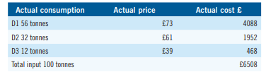
During an eight-hour shift 100 tonnes of product were produced and the actual material content was:
65 tonnes of D1 @ £72/tonne
28 tonnes of D2 @ £61/tonne
11 tonnes of D3 @ £40/tonne
Total input 104 tonnes.
In approaching variance analysis for these more sophisticated situations it is important to identify all the variable factors involved. At a glance it can be seen that the standard and actual prices differ as there are price variances in both D1 and D2.
The actual consumption of raw material tonnage is 104 tonnes for 100 tonnes of product which suggests a yield variance and the mix differs from the standard shown above.
Definitions
These were once defined by CIMA as:
• Direct material mix variance.
Total material input in a standard mix at standard prices less actual material input at standard prices. This is a sub-set of the direct material usage variance applicable where materials are combined in standard proportion. It shows the effect on cost on variations from standard proportion.
• Direct material yield variance.
Standard quantity of material specified for actual production at standard prices less the actual total material input in standard proportions at standard prices.
Example (2)
In a further production period based on the standard mixture shown above, it is assumed that a process loss of 10% is anticipated. During the period output was 81 tonnes and the actual inputs and costs were:
There are five variances to be identified here:
• Direct material cost variance.
• Direct material price variance.
• Direct material usage variance that sub divides to:
• Direct material mix variance and;
• Direct material yield variance.
There are various approaches to this type of problem, the which follows is based on an approach to variance analysis by a former professional associate and late friend Joe Baggott (City of Birmingham Polytechnic), who with his excellent presentations on this topic made learning an enjoyable journey.
The approach is to arrange the data in tabular form using the following key to column headings:
S = Standard
A = Actual
P = Price
Q = Quantity
M = Mixture
Referring to the Example (2) above for a production of 81 tonnes
with a 10% process loss the input would be 81 x 10/9 = 90 tonnes and converted to standard proportions as: (60:30:10) would show: D1 54 tonnes, D2 27 tonnes and D3 9 tonnes.
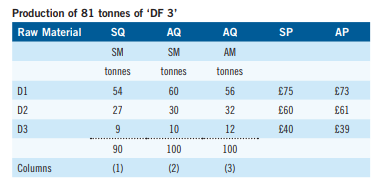
We then evaluate the quantities within the mix shown in columns (1), (2) and (3) above by either standard or actual prices. For example column (A) shown below is from column (1) D1 54 tonnes @£75/tonne = £4050
Direct material cost variance
Column (A) less Column (D)
£6030 – £6508
£478 Adverse
This is the difference between the standard cost of the actual output and the actual cost.
Direct material price variance
Column (C) less Column (D)
£6600 – £6508
£92 Favourable
This is the difference between the standard and actual prices multiplied by the actual quantities.
Direct material usage variance
Column (A) less Column (C)
£6030 – £6600
£570 Adverse
This is difference between the standard usage and the actual usage at the standard prices.
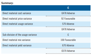
The Direct material then sub-divides to:
• Direct material mix variance
• Direct material yield variance
Mix:
Column (B) less Column (C)
£6700 – £6600
£100 Favourable
This simply identifies the change in the mix – the difference between the standard and actual mix at standard prices.
Yield:
Column (A) less Column (B)
£6030 – £6700
£670 Adverse
This identifies the change in usage to achieve the actual volume of output and is termed the yield.
Having read this overview of these advanced variances please when
preparing for your examination give some thought to what factors may have contributed to the variances shown above.
• Dr Philip E Dunn is a freelance author and technical editor for Kaplan and Osborne Books.
